
Basics of DSP
Discretization of a continuous-time signal (sampling and aliasing)
Consider a continuous-time signal whose Fourier transform is . Then
and
A discrete-time signal can be obtained by uniformly sampling the continuous-time signal at discrete intervals where is called the sampling period and is an integer. Consider a unit impulse function , whose value is at and elsewhere. Then the unit impulse sequence can be expressed as
and can be expressed as
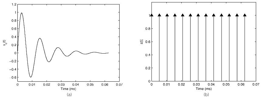
Figure 1:
(a) Damped sinusoid,
(b) Impulse train,
(c) Illustration of sampling and
(d) Sampled signal.
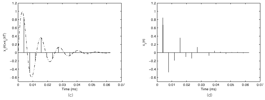
Figure 2: Fourier transform of
(a) Bandlimited signal and
(b) Impulse train.
Discrete time Fourier transform of
(c) Oversampled signal ()
(d) Undersampled signal ().
Figure 1 illustrates the process and effect of sampling a continuous-time signal in the time domain. In the frequency domain, the corresponding Fourier transform of (x_d(n)) can be obtained by convolving the individual Fourier transforms of (x_c(t)) and (s(t)). This is because multiplication of two sequences in the time domain is equivalent to convolution in the Fourier domain. Similarly multiplication in the Fourier domain is equivalent of convolution in the time domain.
To observe the effect of sampling in the frequency domain, we need to consider the Fourier Transform of . Since is periodic with period , using Fourier series expansion it can be shown that
where is the sampling frequency.
Now the Fourier transform of may be computed as
Thus the Fourier transform of an impulse train with period is another impulse train with period . To illustrate the effect of sampling in the frequency domain, consider some arbitrary Fourier transform of a signal with bandwidth shown in Figure 2(a). The Fourier transform of the impulse train sequence with period is shown in Figure 2(b) where denotes the sampling frequency. The corresponding discrete-time Fourier transform of the sampled signal is shown in Figure 2(c) for the case where . If the sampling frequency is reduced (), the resultant discrete-time Fourier transform (shown in Figure 2(d)) clearly indicates the overlapping of spectral components. This effect is called aliasing and is due to an insufficient sampling rate. If the signal is sampled at a sampling frequency of , then no spectral distortion occurs as can be seen from (shown in Figure 3). Hence the minimum sampling frequency required to discretize a signal without aliasing is equivalent to twice the bandwidth of the signal. This frequency is referred to as the Nyquist rate.
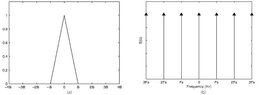

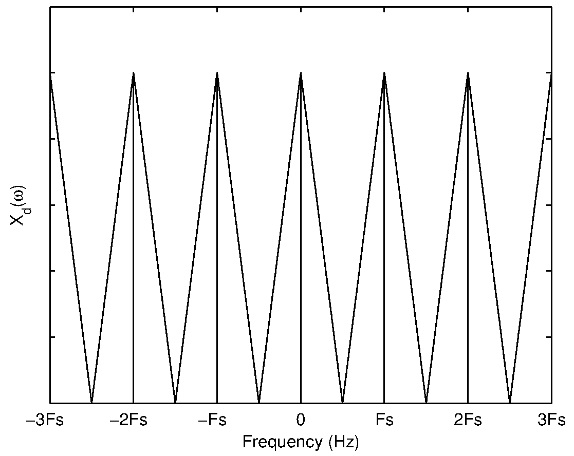
Figure 3: Discrete time Fourier transform of signal sampled at Nyquist frequency
().
A discrete-time signal obtained through sampling is still a continuous amplitude time sequence, where each sample value has an infinite precision. But digital computers are finite precision machines and hence there is a need to discretize and limit the range of sample values. This is achieved by quantization (more accurately scalar quantization). In the quantization process, each sampled value of a discrete-time signal is compared against a finite set of amplitude values and assigned a value in the set that is closest to the discrete-time value. The number of elements in the finite set is determined by the precision of the digital system. In an 8-bit system, there are elements in the set. The number of elements in the finite set is referred as the number of quantization levels. If the difference in values of adjacent elements in the ordered set is constant, then the quantizer is referred as a uniform linear quantizer. Figure 4 shows the effect of quantizing a line using a 3-bit quantizer.
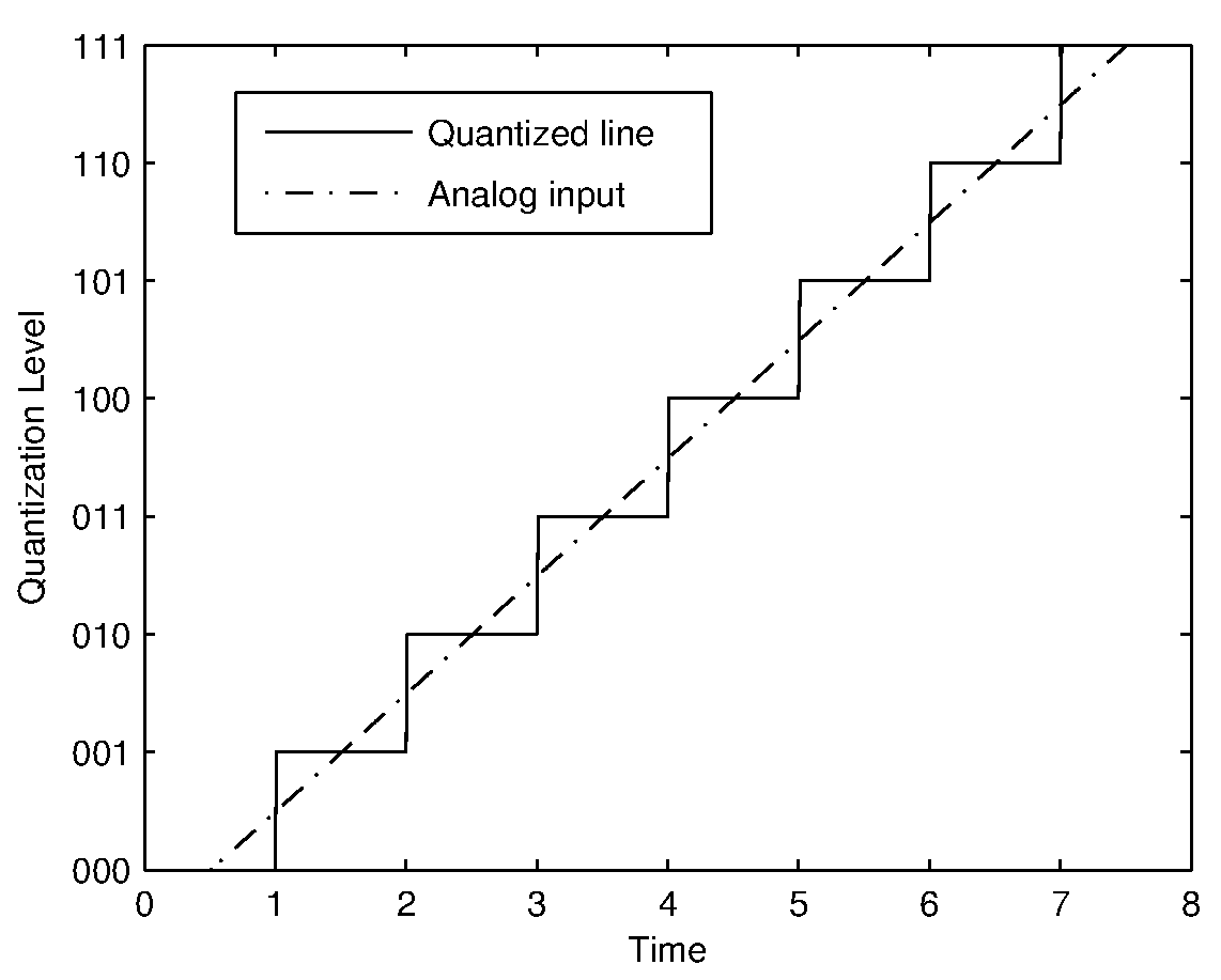
Figure 4: Quantization of a linear segment of an analog signal.
Since the digital signal is obtained by quantizing the continuous valued discrete-time signal, there is an error introduced in representation of the signal. If the discrete-time signal has a limited amplitude range (i.e., ), the quantization step for a -bit uniform quantizer is given by
The maximum quantization error introduced by a -bit uniform quantizer is given by
Hence the quantization error for each sample is defined as
where is the discrete-time infinite precision sampled value of the continuous-time signal , and is the finite precision digitized (sampled and quantized) sample value. The quantization error at each sample lies within the range
A resonator is an all-pole system. The transfer function of an all-pole system is given by
where denote the real coefficients of the denominator polynomial of order . Roots of the denominator polynomial in give real or complex poles. Real roots correspond to zero frequency or . Complex roots of a polynomial with real coefficients always occur in complex conjugate pairs corresponding to a frequency related to the angle of the complex root. Each pair of complex conjugate roots (or poles) corresponds to a second order polynomial which may be denoted as
where the complex root is given by
where denotes the resonance frequency of the second order system, and corresponds to the resonance bandwidth given by
where denotes the sampling interval. By using Eq. 18 and Eq. 19, Eq. 17 can be derived as
where represents the sampling frequency.
For example, the magnitude response of an all-pole system with resonant frequency Hz, Hz and Hz is shown in Figure 5. The impulse response is a sampled sinusoidal signal. The damping depends on the bandwidth of the pole of the system.
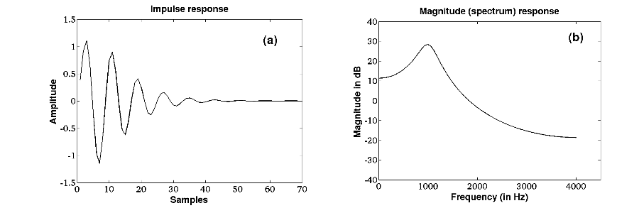
Figure 5: Impulse response and magnitude response.
Consider a train of impulse sequence, , with each impulse located at integer multiples of () as shown in Figure 6. The output resonance of the system is shown in Figure 7. The output signal is periodic with fundamental period () (from which the fundamental frequency is obtained as ) is shown in Figure 7.
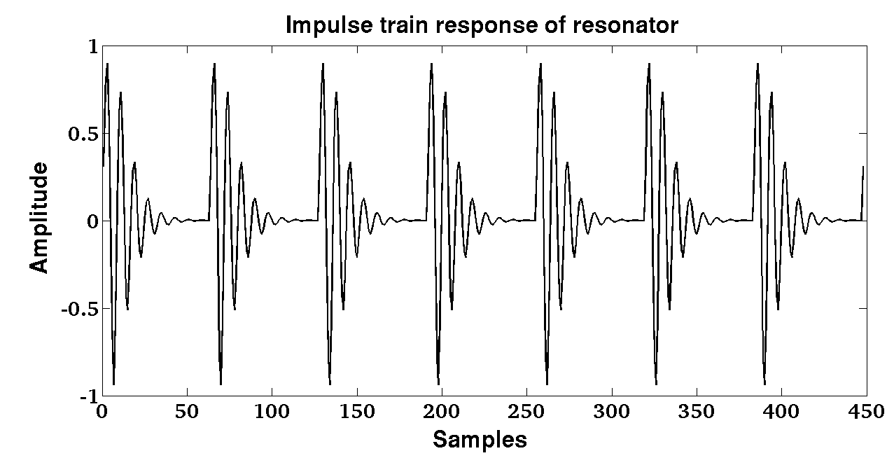
Figure 6: Train of impulse sequence.
Figure 7: Output resonance of the system.